Attention Models in Neural Networks

Attention mechanisms in neural networks, otherwise known as neural attention or just attention, have recently attracted a lot of attention (pun intended). In this post, I will try to find a common denominator for different mechanisms and use-cases and I will describe (and implement!) two mechanisms of soft visual attention.

What is Attention?

Informally, a neural attention mechanism equips a neural network with the ability to focus on a subset of its inputs (or features): it selects specific inputs. Let \(\mathbf{x} \in \mathcal{R}^d\) be an input vector, \(\mathbf{z} \in \mathcal{R}^k\) a feature vector, \(\mathbf{a} \in [0, 1]^k\) an attention vector, \(\mathbf{g} \in \mathcal{R}^k\) an attention glimpse and \(f_\mathbb{\phi}(\mathbf{x})\) an attention network with parameters \(\mathbb{\phi}\). Typically, attention is implemented as

\[\begin{align} \mathbf{a} &= f_\phi(\mathbf{x}), \tag{1} \label{att}\\ \mathbf{g} &= \mathbf{a} \odot \mathbf{z}, \end{align}\]

where \(\odot\) is element-wise multiplication, while \(\mathbf{z}\) is an output of another neural network \(f_\mathbf{\theta} (\mathbf{x})\) with parameters \(\mathbf{\theta}\). We can talk about soft attention, which multiplies features with a (soft) mask of values between zero and one, or hard attention, when those values are constrained to be exactly zero or one, namely \(\mathbf{a} \in \{0, 1\}^k\). In the latter case, we can use the hard attention mask to directly index the feature vector: \(\tilde{\mathbf{g}} = \mathbf{z}[\mathbf{a}]\) (in Matlab notation), which changes its dimensionality and now \(\tilde{\mathbf{g}} \in \mathcal{R}^m\) with \(m \leq k\).

To understand why attention is important, we have to think about what a neural network really is: a function approximator. Its ability to approximate different classes of functions depends on its architecture. A typical neural net is implemented as a chain of matrix multiplications and element-wise non-linearities, where elements of the input or feature vectors interact with each other only by addition.

Attention mechanisms compute a mask which is used to multiply features. This seemingly innocent extension has profound implications: suddenly, the space of functions that can be well approximated by a neural net is vastly expanded, making entirely new use-cases possible. Why? While I have no proof, the intuition is following: the theory says that neural networks are universal function approximators and can approximate an arbitrary function to arbitrary precision, but only in the limit of an infinite number of hidden units. In any practical setting, that is not the case: we are limited by the number of hidden units we can use. Consider the following example: we would like to approximate the product of \(N >> 0\) inputs. A feed-forward neural network can do it only by simulating multiplications with (many) additions (plus non-linearities), and thus it requires a lot of neural-network real estate. If we introduce multiplicative interactions, it becomes simple and compact.

The above definition of attention as multiplicative interactions allow us to consider a broader class of models if we relax the constrains on the values of the attention mask and let \(\mathbf{a} \in \mathcal{R}^k\). For example, Dynamic Filter Networks (DFN) use a filter-generating network, which computes filters (or weights of arbitrary magnitudes) based on inputs, and applies them to features, which effectively is a multiplicative interaction. The only difference with soft-attention mechanisms is that the attention weights are not constrained to lie between zero and one. Going further in that direction, it would be very interesting to learn which interactions should be additive and which multiplicative, a concept explored in A Differentiable Transition Between Additive and Multiplicative Neurons. The excellent distill blog provides a great overview of soft-attention mechanisms.

Visual Attention

Attention can be applied to any kind of inputs, regardless of their shape. In the case of matrix-valued inputs, such as images, we can talk about visual attention. Let \(\mathbf{I} \in \mathcal{R}^{H \times W}\) be an image and \(\mathbf{g} \in \mathcal{R}^{h \times w}\) an attention glimpse i.e. the result of applying an attention mechanism to the image \(\mathbf{I}\).

Hard Attention

Hard attention for images has been known for a very long time: image cropping. It is very easy conceptually, as it only requires indexing. Let \(y \in [0, H - h]\) and \(x \in [0, W - w]\) be coordinates in the image space; hard-attention can be implemented in Python (or Tensorflow) as

g = I[y:y+h, x:x+w]

The only problem with the above is that it is non-differentiable; to learn the parameters of the model, one must resort to e.g. the score-function estimator (REINFORCE), briefly mentioned in my post.

Soft Attention

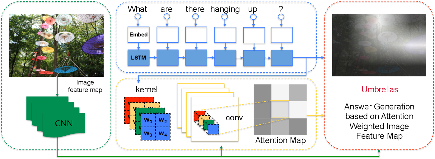
Soft attention, in its simplest variant, is no different for images than for vector-valued features and is implemented exactly as in equation \ref{att}. One of the early uses of this types of attention comes from the paper called Show, Attend and Tell: The model learns to attend to specific parts of the image while generating the word describing that part.

This type of soft attention is computationally wasteful, however. The blacked-out parts of the input do not contribute to the results but still need to be processed. It is also over-parametrised: sigmoid activations that implement the attention are independent of each other. It can select multiple objects at once, but in practice we often want to be selective and focus only on a single element of the scene. The two following mechanisms, introduced by DRAW and Spatial Transformer Networks, respectively, solve this issue. They can also resize the input, leading to further potential gains in performance.

Gaussian Attention

Gaussian attention works by exploiting parametrised one-dimensional Gaussian filters to create an image-sized attention map. Let \(\mathbf{a}_y \in \mathcal{R}^H\) and \(\mathbf{a}_x \in \mathcal{R}^W\) be attention vectors, which specify which part of the image should be attended to in \(y\) and \(x\) axis, respectively. The attention masks can be created as \(\mathbf{a} = \mathbf{a}_y \mathbf{a}_x^T\).

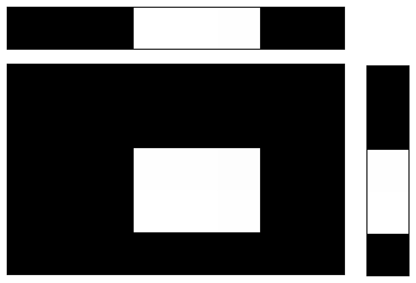In the above figure, the top row shows \(\mathbf{a}_x\), the column on the right shows \(\mathbf{a}_y\) and the middle rectangle shows the resulting \(\mathbf{a}\). Here, for the visualisation purposes, the vectors contain only zeros and ones. In practice, they can be implemented as vectors of one-dimensional Gaussians. Typically, the number of Gaussians is equal to the spatial dimension and each vector is parametrised by three parameters: centre of the first Gaussian \(\mu\), distance between centres of consecutive Gaussians \(d\) and the standard deviation of the Gaussians \(\sigma\). With this parametrisation, both attention and the glimpse are differentiable with respect to attention parameters, and thus easily learnable.

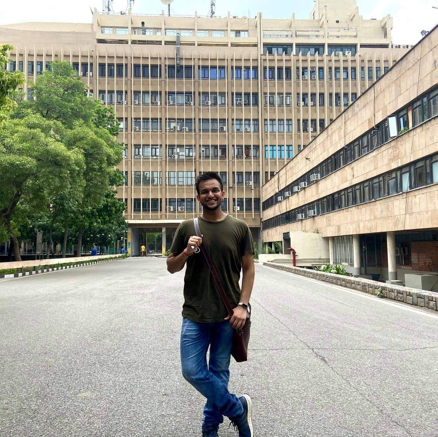
Attention in the above form is still wasteful, as it selects only a part of the image while blacking-out all the remaining parts. Instead of using the vectors directly, we can cast them into matrices \(A_y \in \mathcal{R}^{h \times H}\) and \(A_x \in \mathcal{R}^{w \times W}\), respectively. Now, each matrix has one Gaussian per row and the parameter \(d\) specifies distance (in column units) between centres of Gaussians in consecutive rows. The glimpse is now implemented as

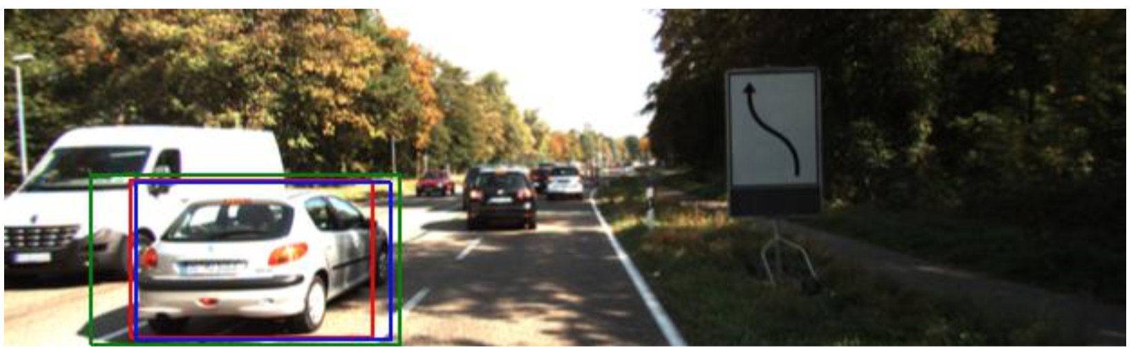
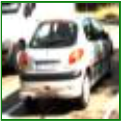
\[\mathbf{g} = A_y \mathbf{I} A_x^T.\]

Here is an example with the input image on the left hand side and the attention glimpse on the right hand side; the glimpse shows the box marked in the main image in green:

The code below lets you create one of the above matrix-valued masks for a mini-batch of samples in Tensorflow. If you want to create \(A_y\), you would call it as Ay = gaussian_mask(u, s, d, h, H), where u, s, d are \(\mu, \sigma\) and \(d\), in that order and specified in pixels.

def gaussian_mask(u, s, d, R, C):
    """
    :param u: tf.Tensor, centre of the first Gaussian.
    :param s: tf.Tensor, standard deviation of Gaussians.
    :param d: tf.Tensor, shift between Gaussian centres.
    :param R: int, number of rows in the mask, there is one Gaussian per row.
    :param C: int, number of columns in the mask.
    """
    # indices to create centres
    R = tf.to_float(tf.reshape(tf.range(R), (1, 1, R)))
    C = tf.to_float(tf.reshape(tf.range(C), (1, C, 1)))
    centres = u[np.newaxis, :, np.newaxis] + R * d
    column_centres = C - centres
    mask = tf.exp(-.5 * tf.square(column_centres / s))
    # we add eps for numerical stability
    normalised_mask = mask / (tf.reduce_sum(mask, 1, keep_dims=True) + 1e-8)
    return normalised_mask

We can also write a function to directly extract a glimpse from the image:

def gaussian_glimpse(img_tensor, transform_params, crop_size):
    """
    :param img_tensor: tf.Tensor of size (batch_size, Height, Width, channels)
    :param transform_params: tf.Tensor of size (batch_size, 6), where params are  (mean_y, std_y, d_y, mean_x, std_x, d_x) specified in pixels.
    :param crop_size): tuple of 2 ints, size of the resulting crop
    """
    # parse arguments
    h, w = crop_size
    H, W = img_tensor.shape.as_list()[1:3]
    split_ax = transform_params.shape.ndims -1
    uy, sy, dy, ux, sx, dx = tf.split(transform_params, 6, split_ax)
    # create Gaussian masks, one for each axis
    Ay = gaussian_mask(uy, sy, dy, h, H)
    Ax = gaussian_mask(ux, sx, dx, w, W)
    # extract glimpse
    glimpse = tf.matmul(tf.matmul(Ay, img_tensor, adjoint_a=True), Ax)
    return glimpse

Closing Thoughts

Attention mechanisms expand capabilities of neural networks: they allow approximating more complicated functions, or in more intuitive terms, they enable focusing on specific parts of the input. They have led to performance improvements in natural language benchmarks, as well as to entirely new capabilities such as image captioning, addressing in memory networks and neural programmers.

I believe that the most important cases in which attention is useful have not been discovered yet. For example, we know that objects in videos are consistent and coherent, e.g. they do not disappear into thin air between frames. Attention mechanisms can be used to express this consistency prior too.