Achieve 31 (Modified Black Jack)

Modified BlackJack: Achieve 31

Assignment 1, COL870 @ IIT Delhi

Modified Blackjack (Achieve 31) using Reinforcement Learning:

We would like to implement and play a Game similar to the Blackjack given in Sutton and Barto (5.3) with some differences in the rules of the game which are mentioned in the Jupyter notebook Achieve31.ipynb

Deatils of the implementation can be found out in the document Report.pdf

State space is described by a tuple <dealer showing card, agent sum, usable 1, usable 2, usable 3>. Refer the report for seeing what ‘usable’ means. The class Environment models the environment and moves to the next state based on the action taken by the agent. The moves of the dealer are simulated as part of the environment model. In the following, a Model-free setting is assumed, i.e., agent does not know the environment model and can act only based on its past experience.

In particular, it contains two public APIs as follows (taking example of python for syntax):

• reset(): Resets the environment and returns initial state of the environment.

  def reset():
    stuff()
    return initial_state
  

• step(): Takes an action and moves to next_state. Returns next_state, reward associated with the transition and done representing end of episode.

  def step(action):
    action_based_stuff()
    return next_state, reward, done
  

Policy Evaluation

Assuming that the agent follows the following strategy: keep on playing until it can reach a sum of 25 or more using its current cards. Once this happens, stick. This policy is identical to the Dealer’s policy.

Following methods are used to evaluate the Q-value function (for each state action pair) using the following methods:

1. Monte Carlo - both first-visit and every visit.
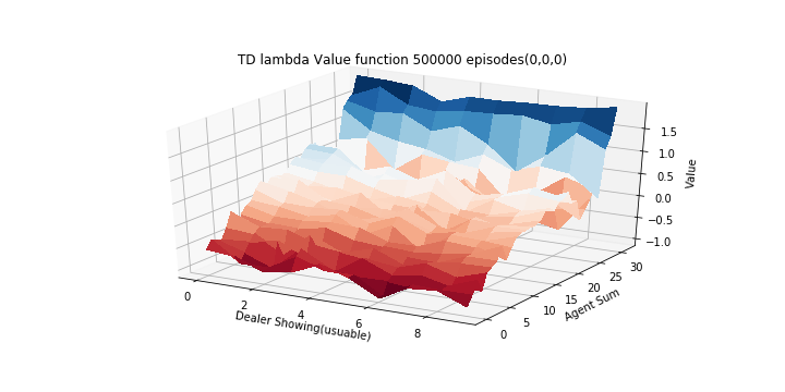
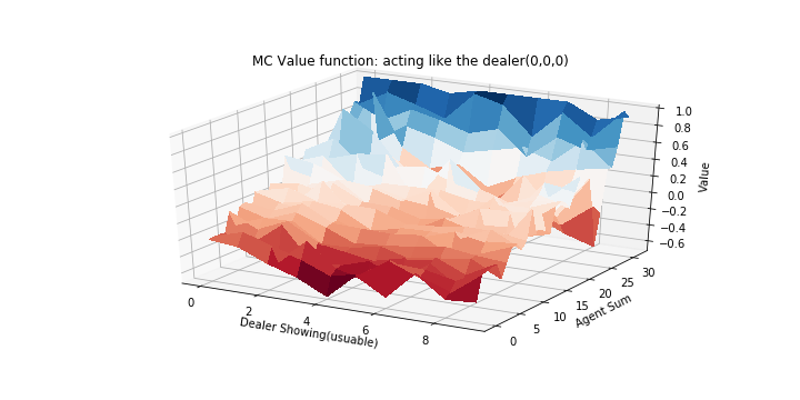
2. k-step TD with values of k going from 1, 3, 5, 10, 100 and 1000. This experiment is repeated after taking averages over 100 runs and 1000 runs in each case. Diagrams similar to the ones used by Sutton and Barto for plotting the value-function are shown below. X-Y plane is used to denote the current state (dealer showing card and agent sum, with 27 different plots for each value of usuables), and Z-axis to denote the value of each state. Following plots are shown for usables (0,0,0)
   • MC every visit:
   • 1 step TD (V averaged over 1000 runs):
   • 1000 step TD (V averaged over 1000 runs):

Policy Control

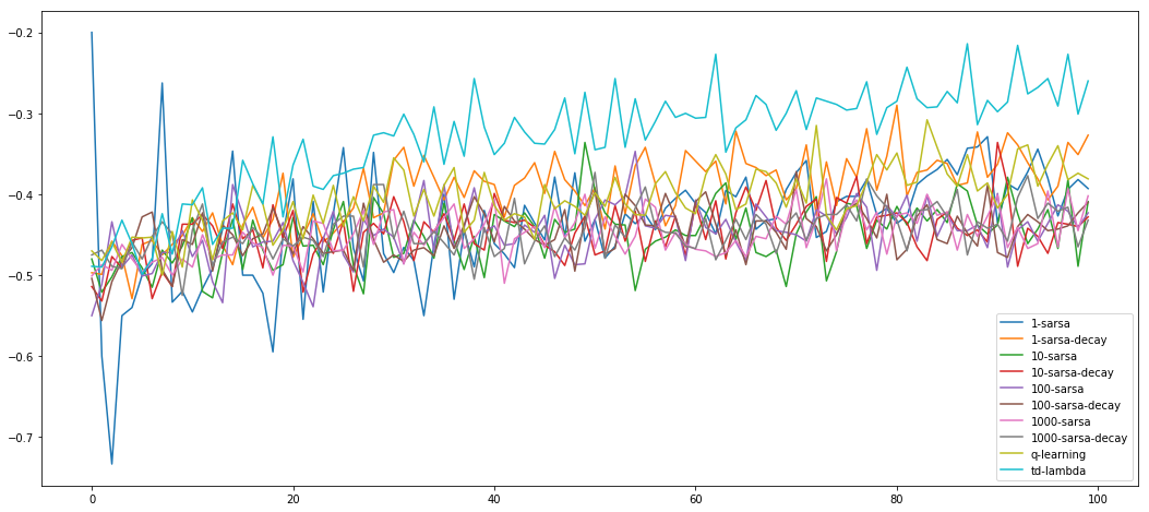
• The following methods are implemented to learn the optimal policy:
  • k-step lookahead SARSA, using an epsilon-greedy policy with a fixed value of epsilon = 0.1 and with k=1, 10, 100, 1000
  • k-step lookahead SARSA, using an epsilon-greedy policy, with k=1, 10, 100, 1000 . Starting with a value of epsilon = 0.1, it is gradually decayed inversely proportional to the number of iterations (i.e., one update corresponds to one iteration)
  • Q-learning with a 1-step greedy look-ahead policy for update and epsilon-greedy policy for exploration in the environment with a fixed epsilon value of 0.1.
  • Forward view of the eligibility traces for TD(0.5) using on-policy control. Epsilon is decayed inversely proportional to the number of iterations starting with a value of 0.1.
• Each algorithm is ran for 100 episodes esing alpha (learning rate) = 0.1. For each algorithm, performance with number of episodes on x-axis and reward (averaged over 10 different runs) on y-axis is shown below.
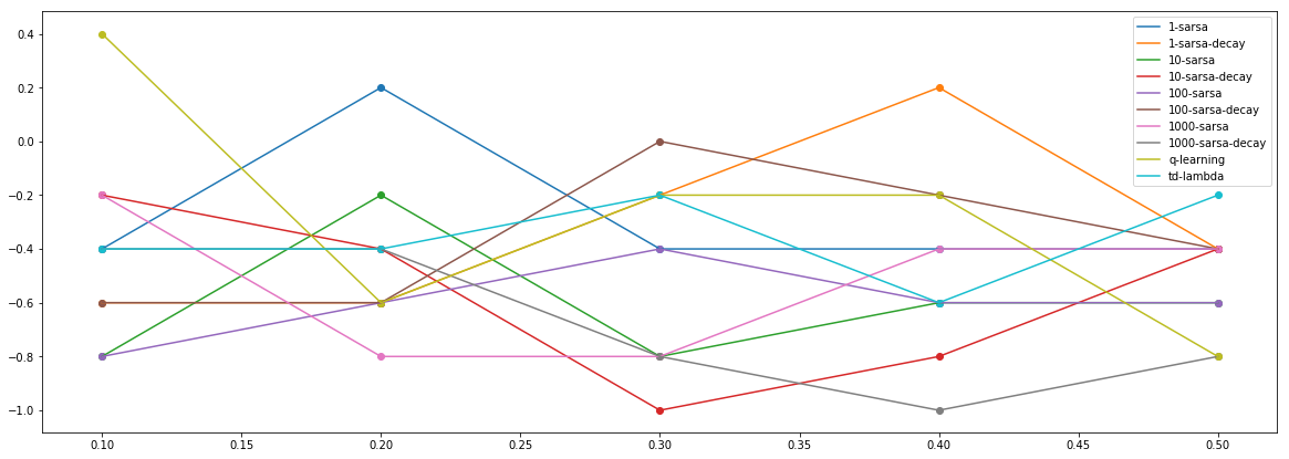
• Each algorithm is then trained for 100,000 episodes. For each algorithm, a set of 10 new (test) episodes is generated by playing the game using the trained algorithm. The performance of each of the algorithms is computed, averaged over this test set. Alpha (learning rate) = 0.1 is used. Next, the entire experiment is reeated by learning the models for alpha values in the set {0.1, 0.2, 0.3, 0.4, 0.5}. The average test performance on y-axis with alpha value on x-axis is shown below.
• The value function for each actionable state for the optimal policy obtained by TD(0.5) with decaying epsilon is shown below.

A detailed explaination of the observations and plots is given in the Report