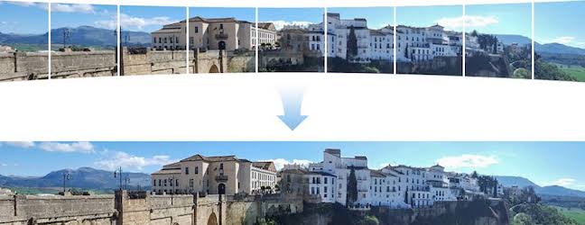
Stitch Panorama of Images

Objective

Brief Description of the approach followed

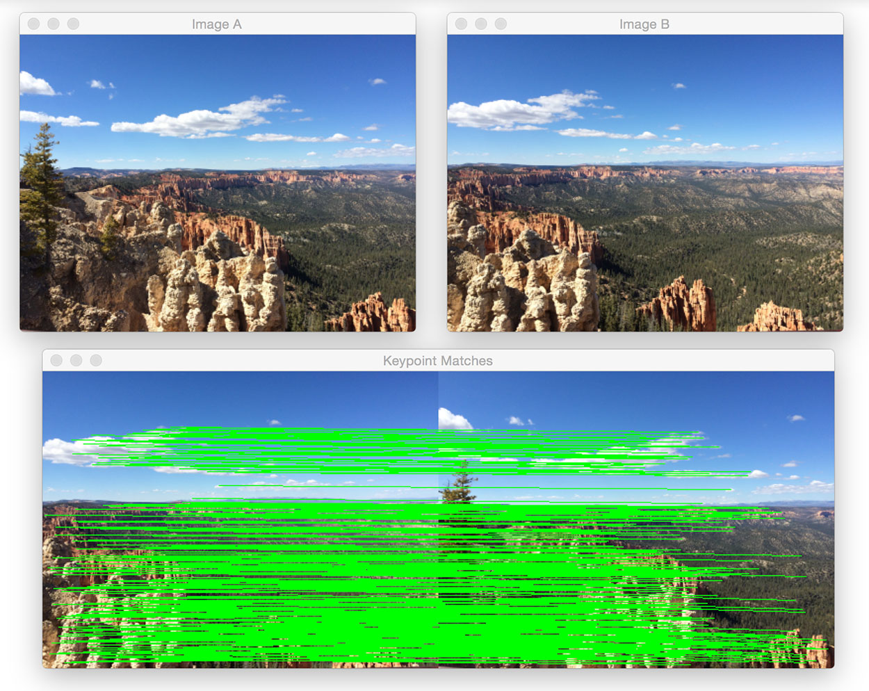
1. Image ​Matching

   • Get each image and compare with the rest one by one.
   • Comparison is done by looking at the similarity in feature points between the two images.
   • Rank the similarity between the images
   • Pairs with low similarity will be discarded, pairs with high enough similarity will be kept.

2. Creating the Panorama

   • After ranking the images in their order and selecting the base image, we first preprocess all the images for basic exposure correction using global histogram equalisation.
   • Images are now resized to a fixed number of rows while maintaining their aspect ratio. This is done to make sure that any two images are always of the same dimension before projection.
   • Compute homographies (H₁, H₂, … H_n) for each image (I₁, I₂, … I_n) with respect to the base image. This homography calculation helps us in estimating the size of final stitched image.
   • Once we have the final size of the stitched image, ​we project each image onto this final estimated screen,​ and compute masks correspondingly to each one of them by appropriate morphological operations. ​Since we do not stitch images one-by-one, our algorithm is robust and works irrespective of vertical/horizontal scene components.
   • We need to make sure that our masks are accurate since our blending procedures are mask-sensitive.
   • Introducing the alpha channel (by adding a 4th channel) in the BGR-image to convert it into appropriate BGRA-image.
   • Blending results performed on the combination of these images have been summarised in a later part, we make use of Enblend package and Laplacian Pyramids. Exposure correction has been properly handled using local histogram equalisation in each window.

3. Blending

   • Different techniques have been experimented with various blending on a sample input test case.
   • Exposure correction has been implemented using ​adaptive/local histogram equalisation​.
   • Here are the results from different implementations.
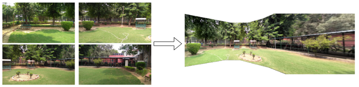
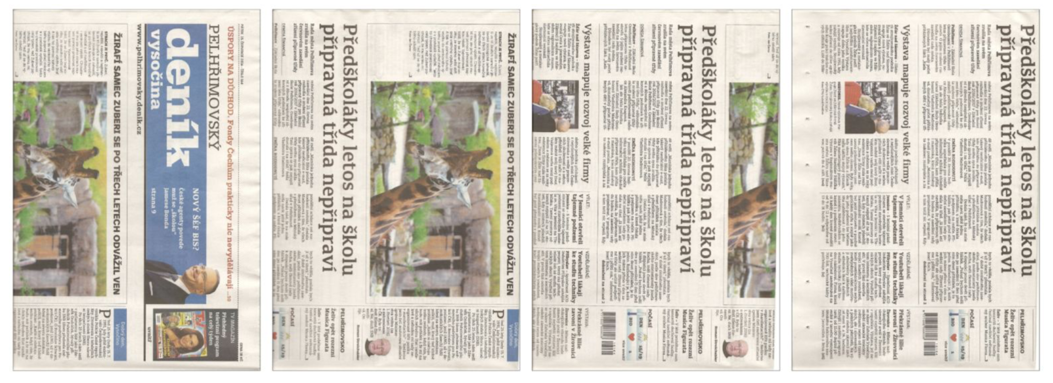
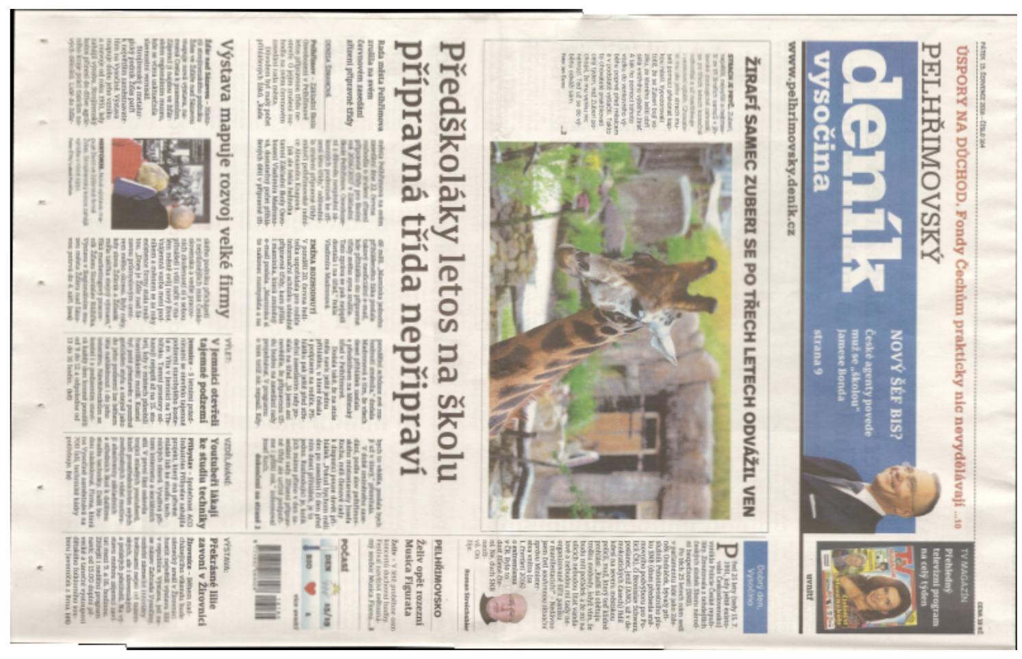
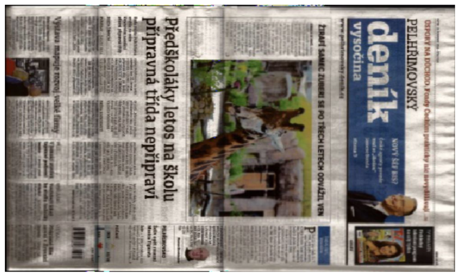
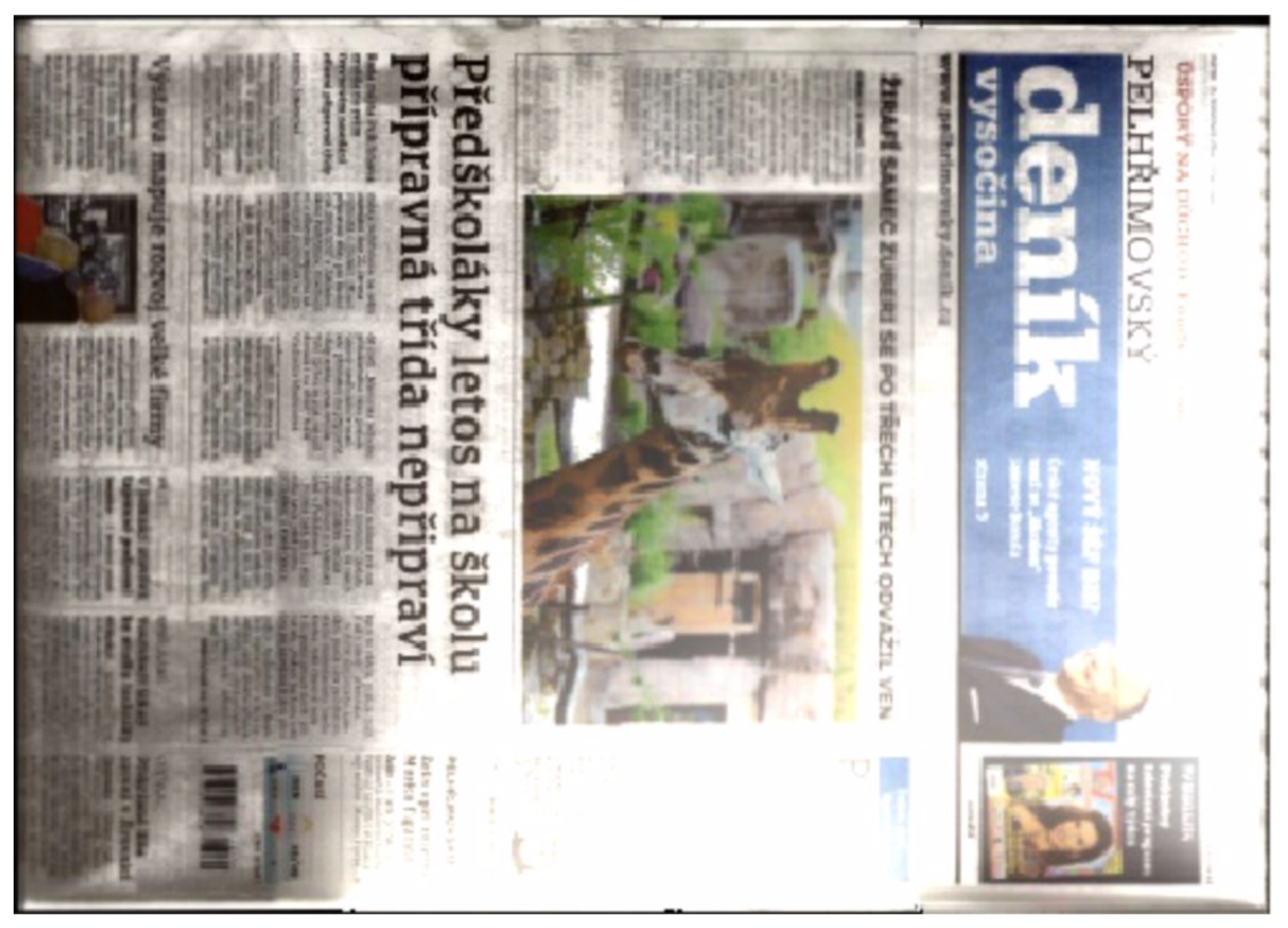
   • Input (Set of 4 Images)
   • Laplacian Blending (with Exposure Correction)
   • Laplacian Blending (without exposure correction)
   • Seamless Blending using Poisson Editing
   • Feathering (Alpha-Blending) - Naive Histogram Equalization
   • Comparison (Alpha Blending v/s Laplacian Blending)

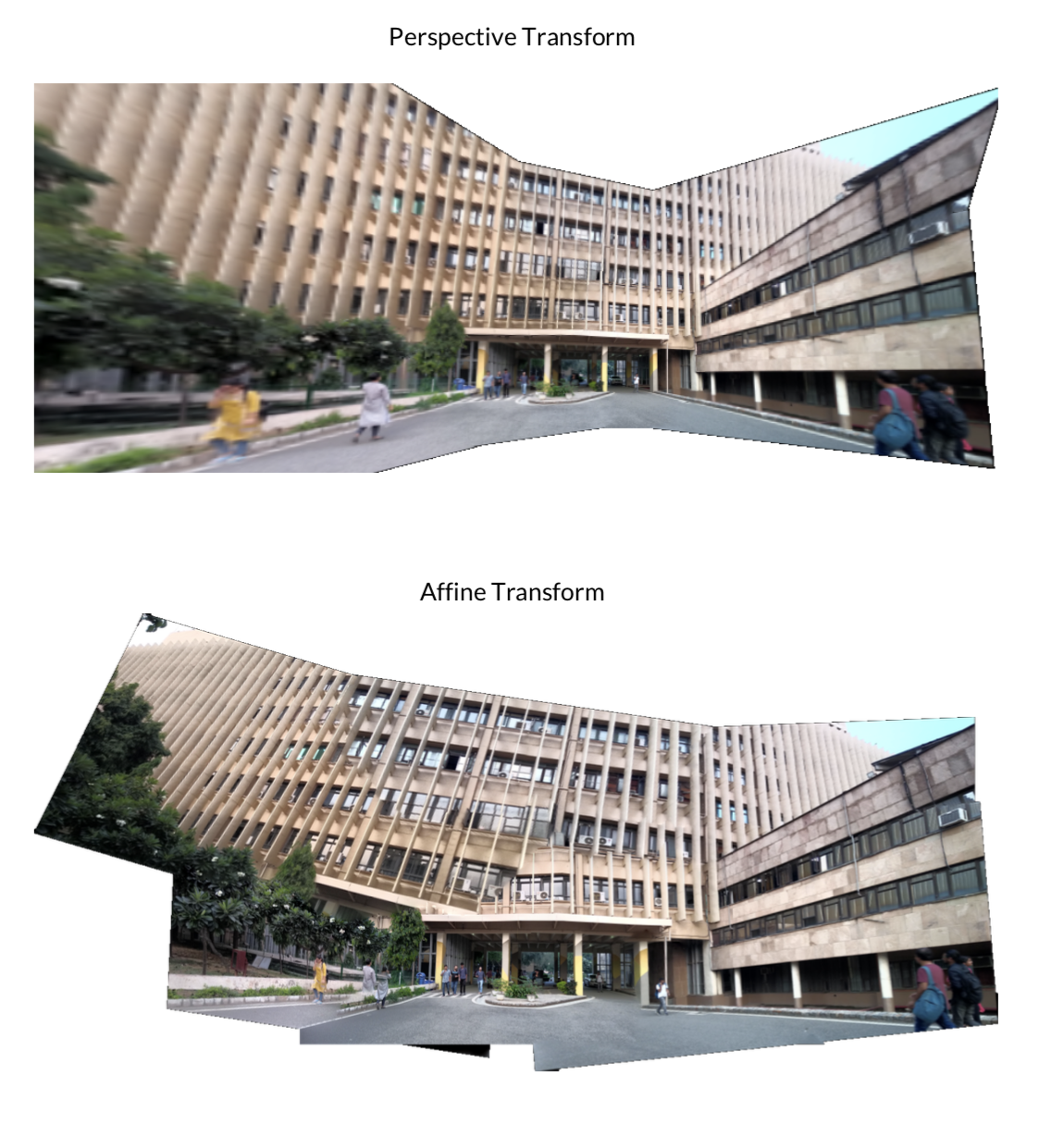
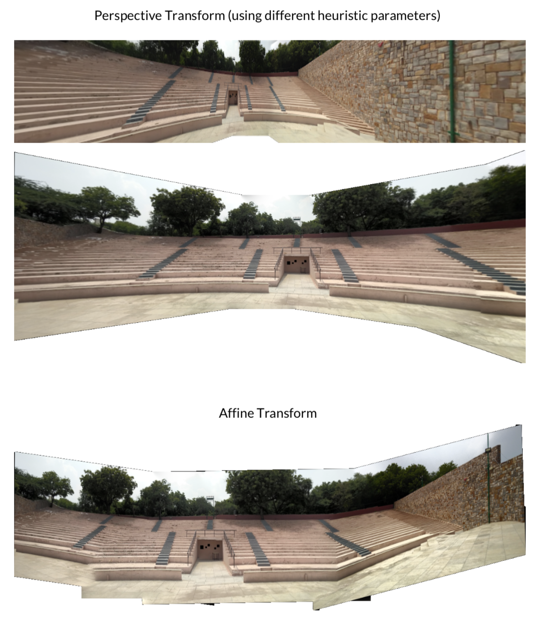
4. Perspective v/s Affine Transform

   • Affine matrix is 2x3, perspective is 3x3; it has less DOF than perspective transformation.
   • Homographic projection maps each point in the first image to the corresponding point of the 2nd image. Straight lines remain straight in a homographic projection, and it can map parallel lines to intersecting lines.
   • An affine projection, on the other hand, transforms the image with respect to the entire image, and this way the parallelism of lines is always preserved.
   • So, if our object is planar but can do out-of-plane rotations, then we need a homography to model that, and in this affine transformation fails since it does not account for out-of-plane transformations.
   • For affine​, we used ​cv.estimateAffine2D to perform only ​rotation​ and t​ranslation​ strictly)
   • Using cv.estimateAffinePartial2D gives better results ​(since it includes s​caling as well)​
   • 
   • 

Our algorithm works regardless of the orientation of supplied images i.e. vertical or horizontal, it does not need an order to be given. As long as the collective set represents a scene,our algorithm works.

Other results have been mentioned in this link along with a comprehensive report.