Probabilistic Graphical Models on a Robotic agent

This is done as part of the course assignment for COL-864 (Robotics Vision) under Prof. Rohan Paul. Assignment Statement is given here.

State Space

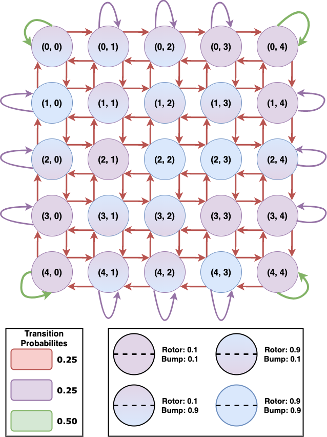
Here, the state space refers to all the possible valid positions in the 2D Grid (5x5) where the agent can possibly be. Each position is a tuple of the form (i, j) representing the ith row and the jth column of the board. This is also made clear from the diagram above. We will use Xt to unique denote the position of the agent (i.e. the state) at the time ‘t’. The set of all possible states is denoted by the symbol S. Hence, the entire state space consists of M2 states where M is the grid size. Hence, in this part, there are 25 states.

S = {(i, j): 0 ≤ i ≤ 4, 0 ≤ j ≤ 4; i, j 𝞊 N}

Observation Space

Since the position of the agent is not visible from the surface of the lake, we use sensors that emit two sounds coming from the Rotor and Bump. Each sound detected by the sensor is a boolean variable indicating the presence or absence of the sound. Hence, the entire observation space is a tuple of 2 boolean variables Bt and Rt. Hence, it consists of four different observations at each time step. The set O completely describes the observation space. We will assume that the state sequence starts at t = 0; for various uninteresting reasons, we will assume that evidence starts arriving at t = 1 rather than t = 0.

B = {“bump”, “no bump”} R = {“rotor”, “no rotor”} O = {(Bi, Rj): Bi 𝞊 {“bump”, “no bump”}, Rj 𝞊 {“rotor”, “no rotor”}}

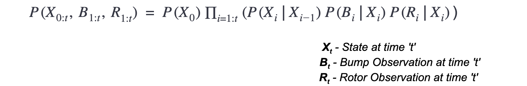
We will use Bt and Rt to denote the observation taken from the sensor at some time ‘t’.

Action Space

It refers to the space of all possible actions taken at each state. As given in the question, the agent is likely to take all the four possible sections {UP, DOWN, LEFT, RIGHT} with an equal probability. If the agent is at a corner position, some of the actions won’t be feasible in that state, but the agent won’t know about it before execution. As a result, the agent won’t change its state, but the action will still be sampled from the same uniform distribution. At will denote the action taken by the agent at a time ‘t’.

A = {UP, DOWN, LEFT, RIGHT}

Transition Model

It refers to modeling the distribution of P(Xt|Xt-1) where Xt denotes the state of the agent at the time ‘t’. Fig below denotes all possible transitions and completely describes the transition model.

All possible transitions within the state space and the spatial likelihood of observations

Observation Model

The probabilities P(Rt | Xt) and P(Bt | Xt) have been shown below respectively. Dark regions denote 0.1 probability while the light regions denote 0.9 probability.

All possible transitions within the state space and the spatial likelihood of observations

Probabilistic Graphical Model (PGM)

Bayesian Network showing the causal cause-effect relationships

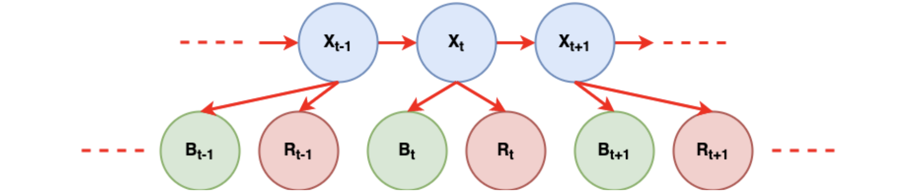
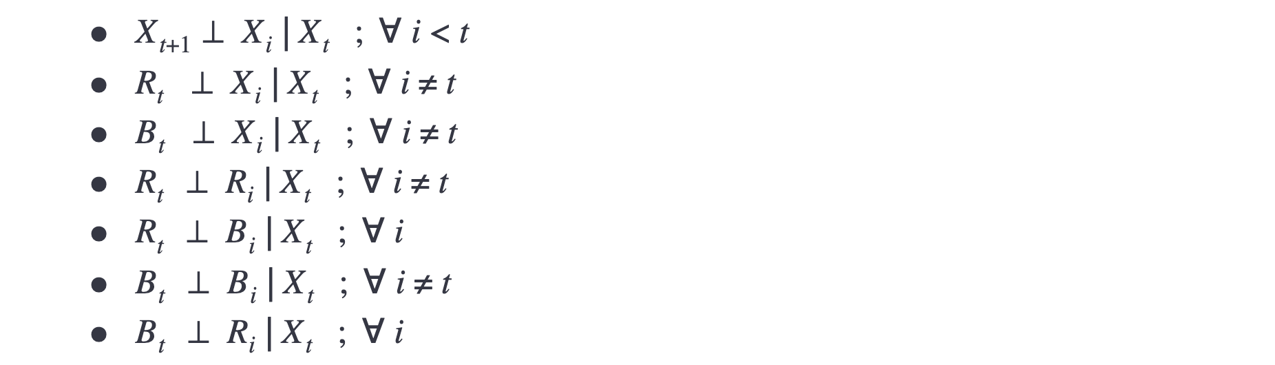
Conditional Independence Assumptions

Joint Distribution

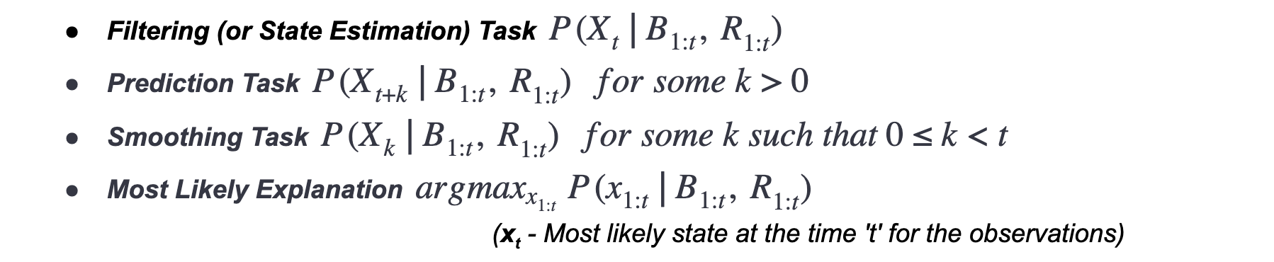
Inference Task

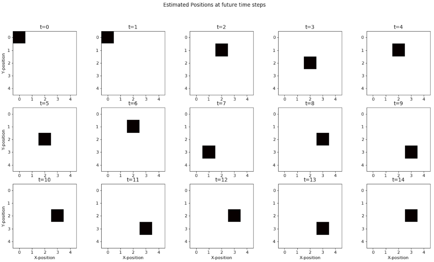
Simulating the agent for 10 timesteps

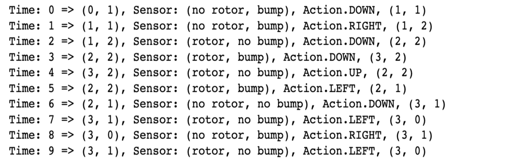
Ground Locations

Filtering Task

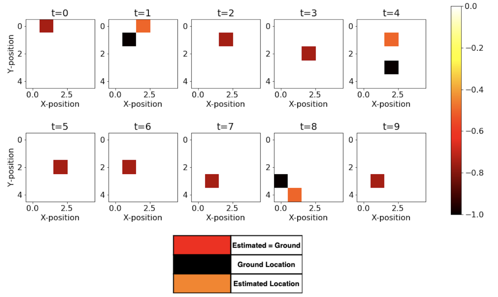
Log-Likelihood of the normalized probabilities estimated for each state by filtering task

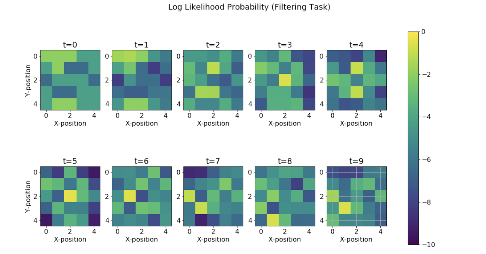
We see how the maximum log-likelihood gives a good estimation of the position of the agent at each time step. We see that there are some mispredictions initially but as soon as we are able to collect more and more evidence and observations from the rotor and bump, we are able to improve the estimation.

Estimated v/s Actual Location at each timestep (Both the Observations)

Dynamic visualization of the movement of the agent

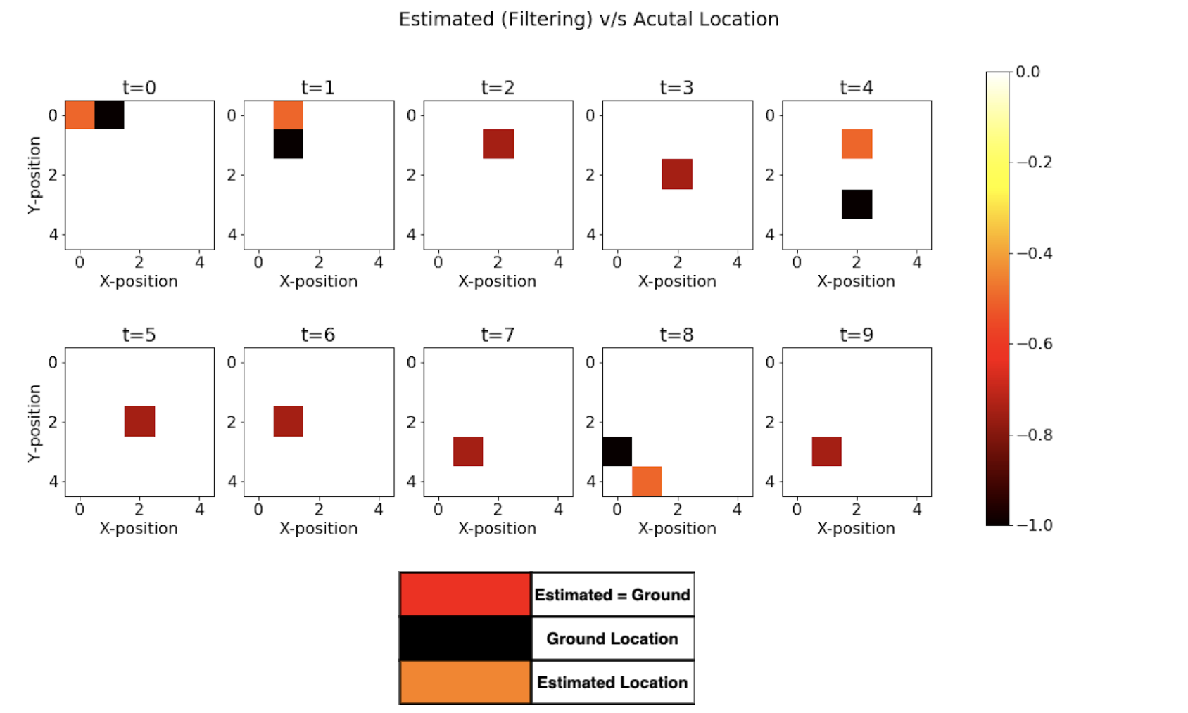
As we see from Fig above, we are able to accurately predict using 6 out of 10 times. We will later see how this result compares using only a single observation and using backward smoothing.

Filtering using only Single Modality

We repeat the same experiment as above but only with a single modality this time. We keep only bump observation (“bump” or “no bump”) as a signal for forwarding filtering.

Log-Likelihood of the normalized probabilities estimated for each state (ONLY bump)

Estimated v/s Actual Location at each timestep (ONLY bump observations)

Dynamic visualization of the movement of the agent (ONLY bump observations)

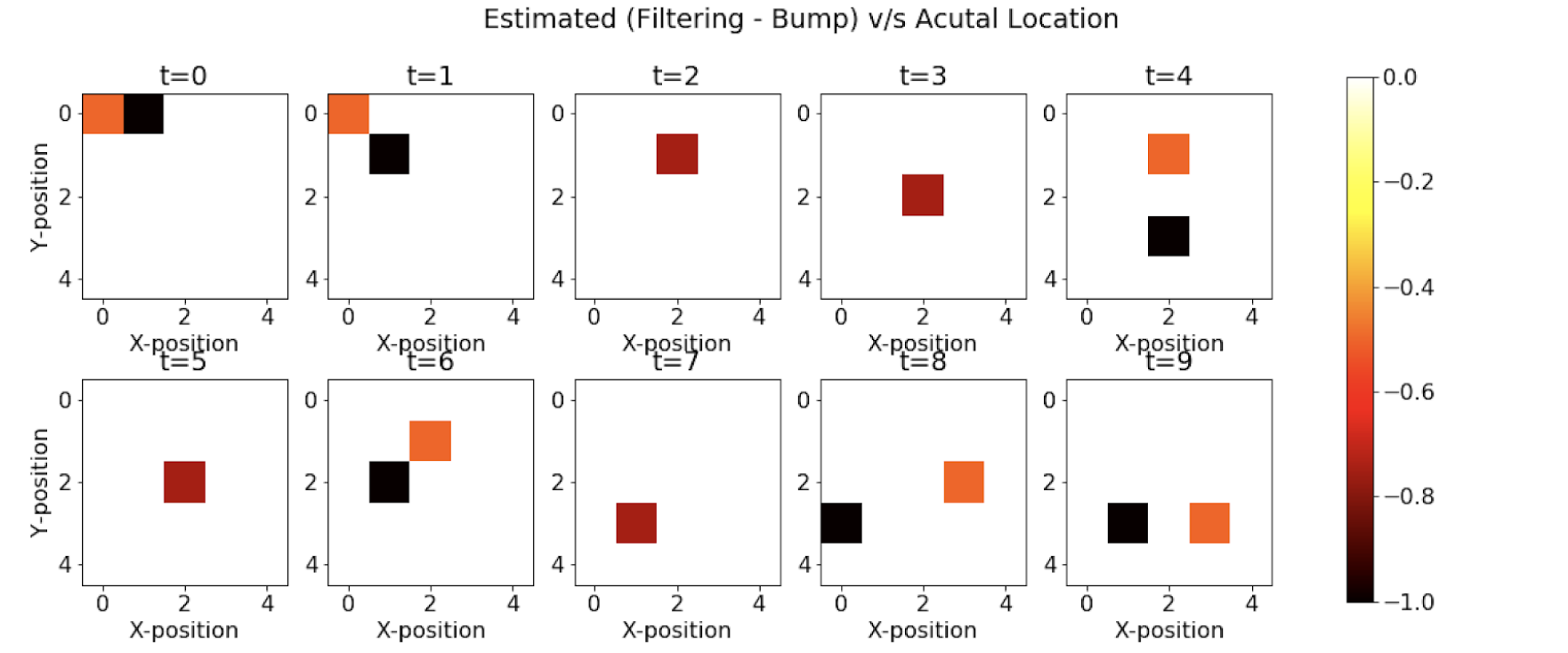
We see that using only bump observations, we are getting more mispredictions since we are using less evidence available. Now, we are able to see only 4 cases (out of 10) when we are accurately able to predict the agent’s position.

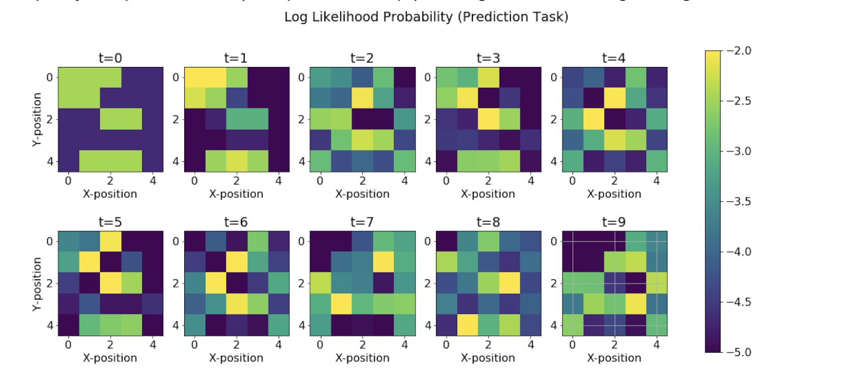
Prediction Task

This is the task of computing the posterior distribution over the future state, given all evidence to date.

Prediction log-likelihood probabilities at the next time step (t = 10) using all evidence

Prediction log-likelihood probabilities at the next 5 time steps using all evidence

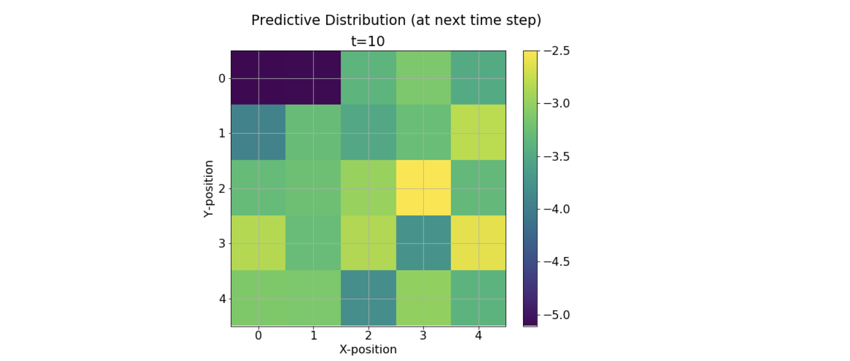
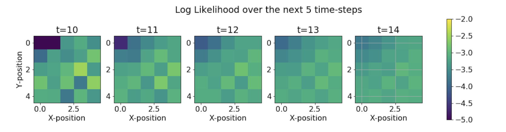
We see that the range of the colormap reduces as the time steps increases. This means that as we try to predict more and more about the future states using the current evidence, we are losing our confidence in the predictions, leading to a decrease in the probability bandwidth. This leads to uncertainty in the state predictions.

Prediction state estimates at all the time steps (0 to 14)

We see an increase in the uncertainty in the movement of agent at the future time steps. The agent merely oscillates around the location at the 10th time step and this uncertainty reaches its peak at the 15th time step.

Smoothing Task

Estimated v/s Actual Location at each timestep (Smoothing Task)

We see from Fig above that the backward algorithm actually helps in fixing the prediction at t = 0 by making use of the future evidence. Now, we see that there are 7 cases out of 10 that are accurately able to estimate the correct position. Fig below shows the dynamic gif representing the movement of the agent and the estimated prediction from the maximum log-likelihood predictions. The improvement in predictions is clearly realized as expected from the Backward Algorithm.

Dynamic Estimated v/s Actual Location at each timestep (Smoothing Task)

Most Likely Explanation (Viterbi Algorithm)

Estimated v/s Actual Location at each timestep (Viterbi Algorithm)

Dynamic Estimated v/s Actual Location at each timestep (Viterbi Algorithm)

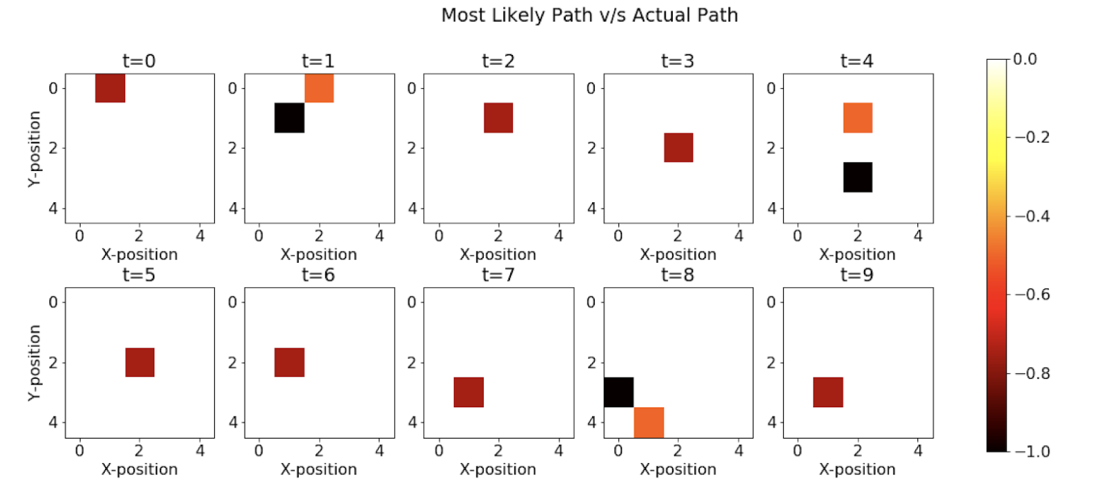
Here, we see that the Viterbi algorithm also performs much better and is accurately able to estimate states correctly 7 out of 10 timesteps. In the implementation, we use a dynamic programming-based approach, and we try to maximise the probability of generation of each state. At each step in the algorithm, we keep a track of the index and then we later backtrack it using the index to find the optimal path of states responsible for this set of observations.

Computing Error

Manhattan Error between two points (a, b) and (x, y) is defined as |a - x| + |b - y|. Here, I have computed this error at each time step and later plotted it to compare the increase.

Manhattan Error between the Actual & Most Likely Path

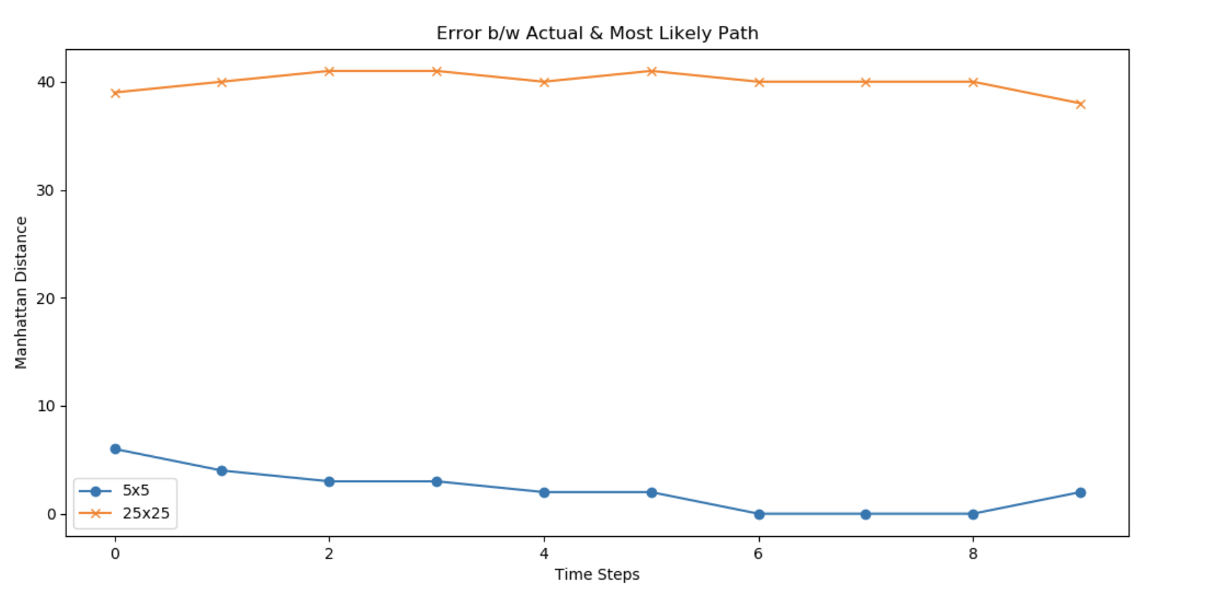
Number of time frames in consideration = 10 Sum of Manhattan error for 5x5 grid size = 22 Sum of Manhattan error for 25x25 grid size = 400

Relative increase in Error = 400/22 = 18.18 Average error per time step (5 x 5) = 2.2 Average error per time step (25 x 25) = 40

The theoretical complexity of the Viterbi Implementation using DP (Source: here) is O(\(T \times |S|^{2}\)). Hence, the computation scales to the 2nd power of the size of state space in consideration. Given T = 10, and \(S_{1}\) = 5 and \(S_{2}\) = 25, we estimate the theoretical increase to be proportional to the ratio of their squares. Hence, theoretically speaking, we should obtain a relative computation complexity of 25.